⚡️ Review lessons of Communication Principles 2 released on my bilibili channel

This is the recording of the review lessons of Communication Principles 2 released on my bilibili channel.
Bilibili:
Communication Principles Final Review – Digital Communication
From Analog to Digital
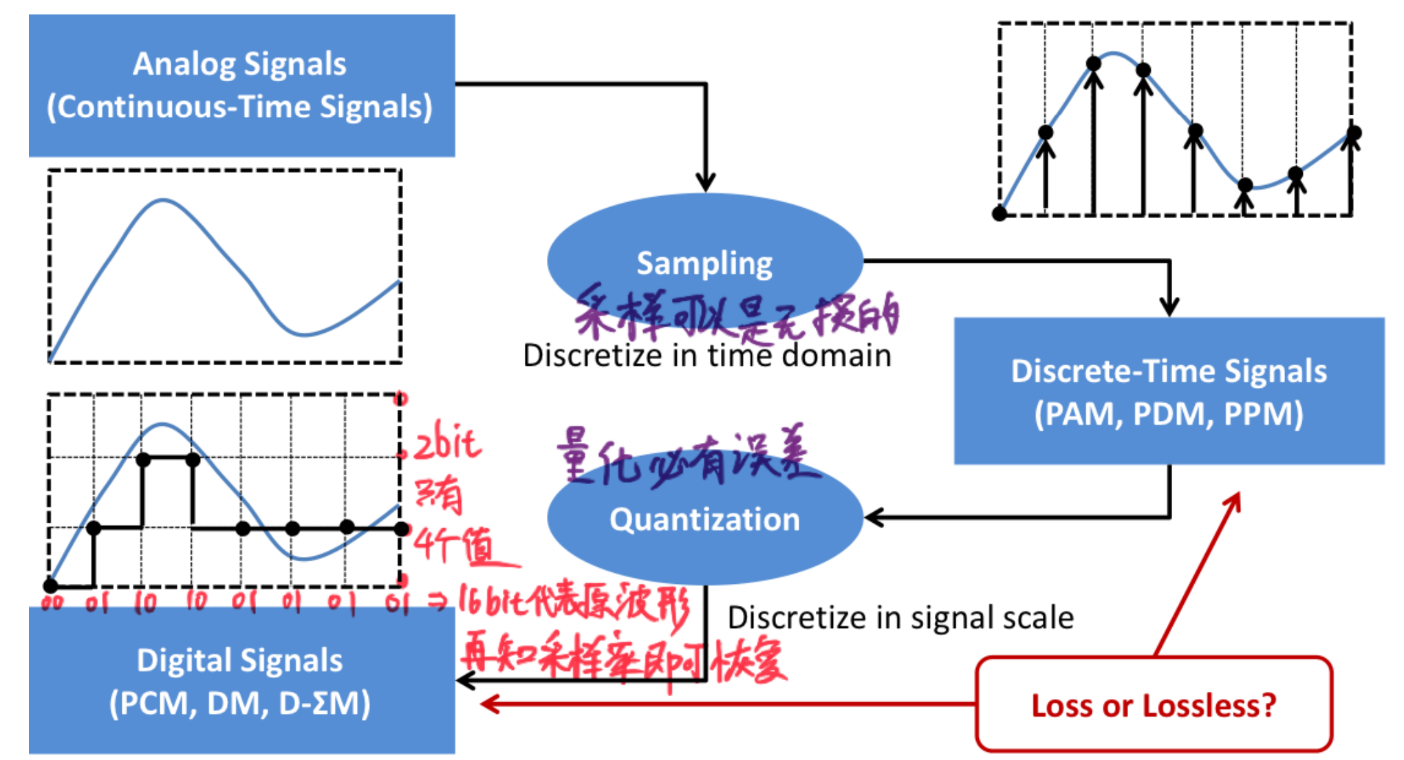
ATTENTION: This discussion is from the receiver’s perspective.
In reality, signals (electromagnetic waves) are continuous. However, our computers can only process discrete data, so it is necessary to convert continuous signals into discrete data. We learned about sampling in signals and systems, but after sampling, the signal is only discrete in time and remains continuous in amplitude, so we need to quantize it. However, ideal sampling is difficult to achieve, and we use Pulse Amplitude Modulation (PAM) and other pulse modulation techniques to approximate sampling.
Sampling
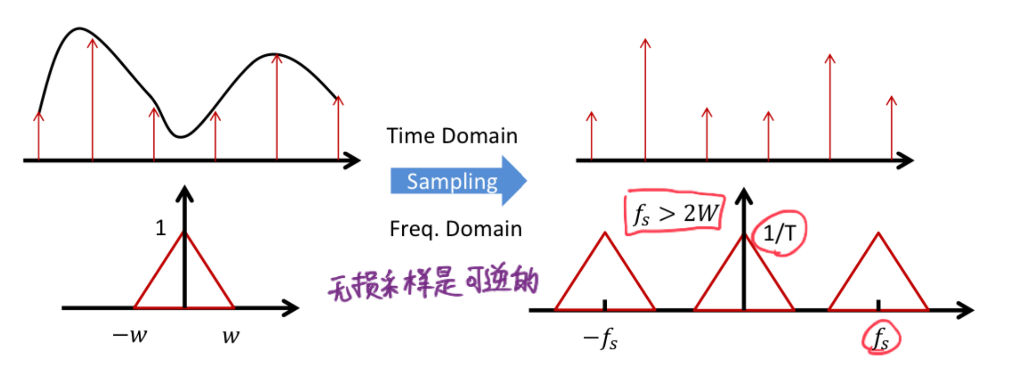
Similar to what we learned in signals and systems, for signals with limited bandwidth, lossless sampling follows the Nyquist theorem, which states that the sampling frequency must be greater than twice the highest frequency of the signal to ensure that the sampled signal is consistent with the original signal.
$$ f_s>2f_{max} $$The sampling function is:
$$ x_s(t)=x(t)\sum_{n=-\infty}^{\infty}\delta(t-nT) $$Where:
$$ T=\frac{1}{f_s} $$The spectrum after sampling is:
$$ X_s(f)=\frac{1}{T}\sum_{n=-\infty}^{\infty}X(f-nf_s) $$Analog Pulse Modulation
Pulse Amplitude Modulation (PAM)
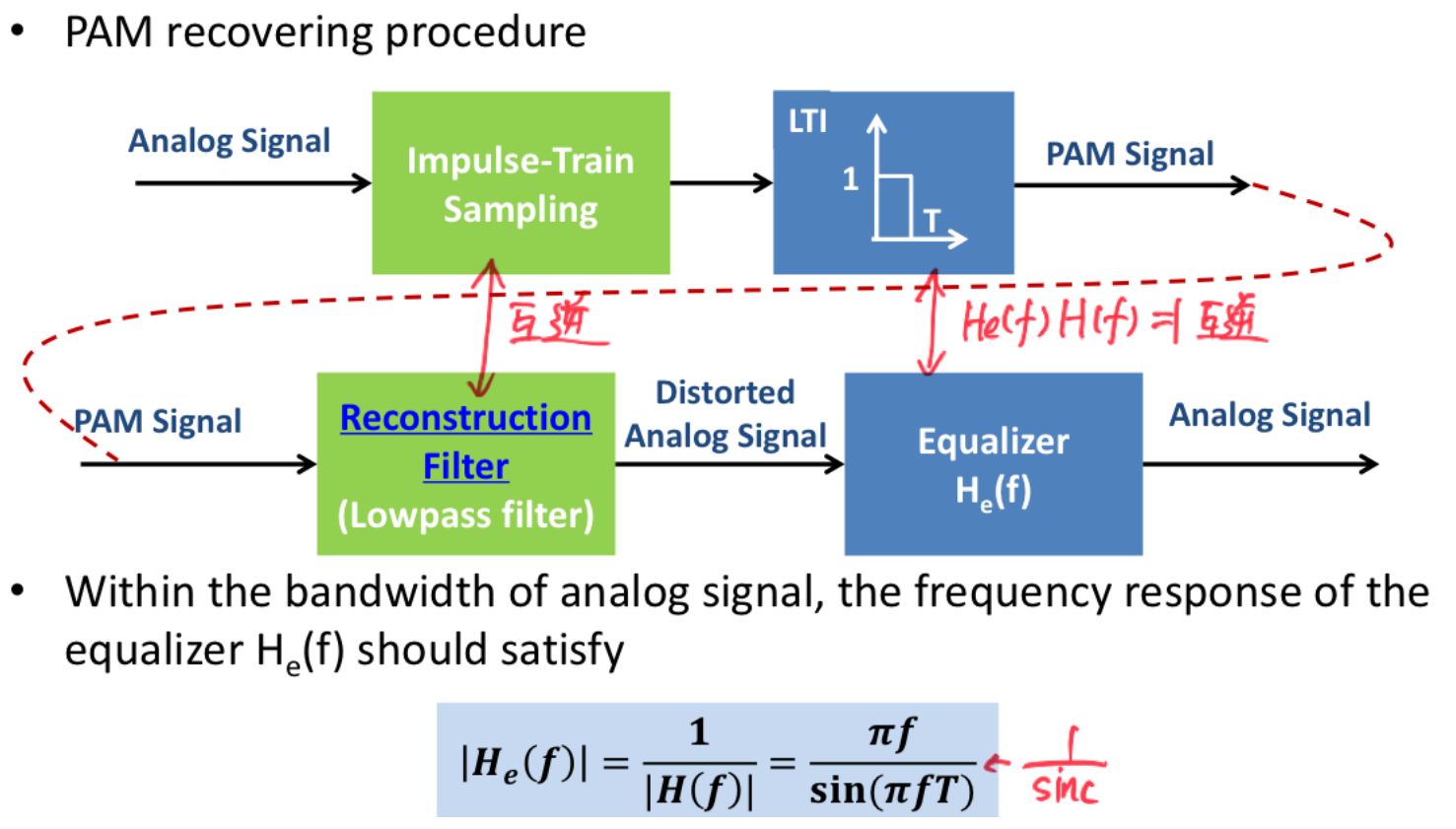
Ideal sampling has an infinitesimally short duration for each point, which is unrealistic. In practical sampling, the sampled signal lasts for a short duration and thus becomes PAM. Its mathematical expression can be understood as the sampling function multiplied by a rectangular pulse, expressed as:
$$ x_{pam}(t)=x(t)\sum_{n=-\infty}^{\infty}\delta(t-nT_s) * [u(t)-u(t-T)] $$The expression for the rectangular function in the frequency domain is:
$$ |H_e(f)|=\frac{1}{|H(f)|}=\frac{\pi f}{\sin(\pi fT)} $$It can be seen that the cost of doing this is the need to occupy a wider bandwidth.
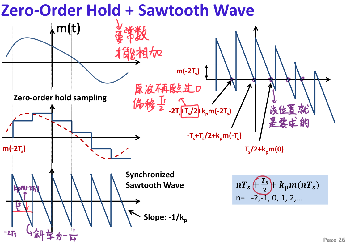
Pulse Position Modulation (PPM)
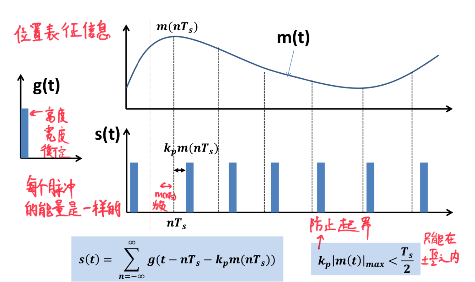
There will be further explanation on how PPM is implemented and how it is demodulated. This part is just to indicate that this method is feasible, and the specific details can be checked later. The most important thing to know is that the purpose of Pulse Modulation is ultimately to convert the amplitudes of the sampling points into a solvable mathematical expression.
At this point, we have achieved a more realistic “sampling,” obtaining the amplitude of each sampling point, but these amplitudes are still continuous. We need to convert them into discrete data; this is quantization.
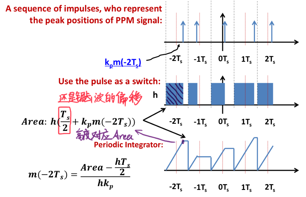
PPM Signal Generation
PPM Detection
-
Determine the position of the Peak
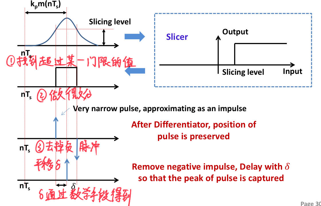
- The shift distance is obviously related to the chosen threshold
-
PPM -> PAM
- The midpoint is the zero point of PPM, so it needs to add Ts/2, which is consistent with the generation of the PPM signal.
Noise Effect in PPM
It is nearly impossible to test, review if you have time.
Quantization
Uniform Quantization
Through the previous steps, we can already obtain the amplitude of each sampling point, but these amplitudes are still continuous. We need to convert them into discrete data; this is quantization. This part is consistent with digital circuits.
- Let L be the number of quantization levels, that is, the number of quantized amplitudes. $L=2^R$, where R is the number of quantization bits.
- The interval between each two quantization levels, known as the quantization step (quantum) (we only discuss the case of uniform quantization): $$ \Delta=\frac{2m_{max}}{L}【m_{max} is the maximum amplitude in the signal】 $$ We assume that the quantization error is uniformly distributed, then: $$ Q \sim U(-\frac{\Delta}{2},\frac{\Delta}{2}) $$ Thus, the mean square value of the quantization error is: $$ E[Q^2]=\frac{\Delta^2}{12} $$ This value is also the power of the quantization error; hence the signal-to-noise ratio (SNR) is: $$ SNR=\frac{P_s}{P_e}=\frac{E[M^2]}{E[Q^2]} =\frac{12P}{\Delta^2}=\frac{3P}{m_{max}^2}2^{2R} $$ It can be observed that the larger the number of quantization bits, the greater the signal-to-noise ratio, but as the number of quantization bits increases, the required bandwidth also increases, so we need to balance between the signal-to-noise ratio and bandwidth.
Nonuniform Quantization
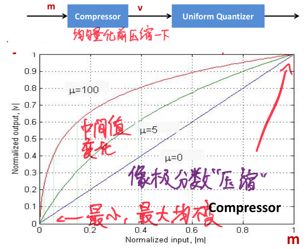
The interval between each quantization level is no longer fixed. If a certain signal amplitude is likely to appear in a specific range, it is reasonable for it to have a higher probability of being quantized to a certain value. The specific implementation can be likened to a type of companding technique: taking the square root of the obtained value and then multiplying it by 10. Of course, the method is not unique. You can understand the $\mu-law$ presented in the course material, but there is no need to memorize the formula.
Example problem: #D3-2
Show that, with a non-uniform quantizer, the average power (mean-square value) of the quantization error is approximately equal to $(1/12)\sum_i{{\Delta_i}^2\mathrm{p_i}}$ where $\Delta_i$ is the i-th step size and $p_i$ is the probability that the input signal amplitude lies within the i-th interval $R_j$. Assume that the step-size $\Delta_i$ is small compared with the range of input signal, such that the signal can be treated as uniformly distributed within each step size.
Hints:
- Let Q be the quantization error, the expectation of Q is given by $E[Q^2]=\sum_i E[Q^2|\text{signal is in the i-th step size}] \Pr [\text{signal is in the i-th step size}]$
- The mean and variance of a uniformly distributed random variable within [a,b] are given by $\frac{1}{2}(a+b)$ and
Pure reading comprehension + statistical questions
At this point, we have obtained purely digital signals!
PS: There is no need to consider Delta Modulation
Baseband Transmission of Digital Signals
The term baseband refers to signals that have not undergone up-conversion, meaning they are generally the most “primitive” signals. Wired communication can directly transmit baseband signals, while wireless communication requires that the signals undergo up-conversion to be transmitted.
A considerable amount of mathematical knowledge is covered here, and we just need to roughly understand and memorize it; familiarity will come with exposure.
Overview
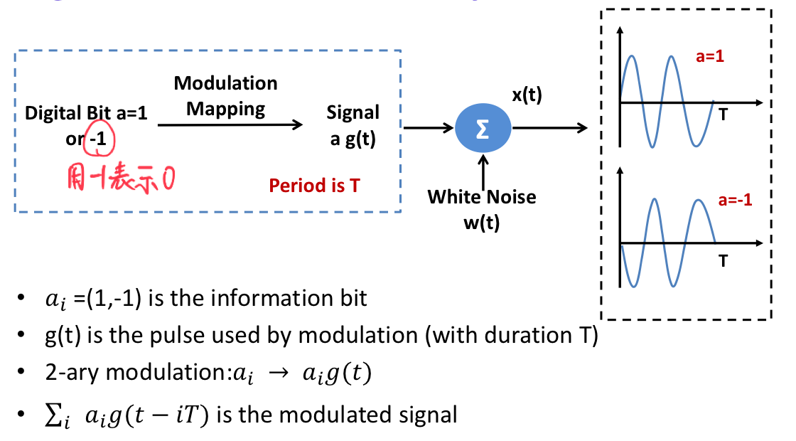
Initially, a device will generate the bit stream that needs to be transmitted. This bit stream is then modulated and converted by the digital-to-analog converter (Modulation Mapping) to obtain the baseband signal. It is then transmitted over a channel. The signal is received by the receiver, which first undergoes [LTI Filter](#LTI Filter), [analog-to-digital conversion](#From Analog to Digital), and demodulation mapping (Demodulation Mapping), and then the bit stream is obtained.
Mathematical Knowledge
Random Process
My understanding combines time series with statistical models. A “process” refers to a function of time. The value at each moment is unpredictable but conforms to a certain distribution.
In other words, if $g(t)$ is a random process, then $g(t_1)$ is a random variable.
ATTENTION: Here we are always addressing an unknown signal. If it is known, such as $g(t)=\sin(t)$, it is determined, and there is no concept of a random process.
Question: If the transmitted signal is known, why is there still a need for a random process?
Answer: The main purpose is to model noise.
Gaussian Process
At any moment $g(t_n)$ of a random process, it is a random variable that follows a Gaussian distribution (normal distribution).
$$ f(x) = \frac{1}{\sqrt{2\pi}\sigma}e^{-\frac{(x-\mu)^2}{2\sigma^2}} $$- For a Gaussian process $g(t)$:
- $g(t_1)$ is a Gaussian random variable
- $a_1g(t_1)+a_2g(t_2)$ is a Gaussian random variable
- For a known function $f(t)$, $\int_{t_1}^{t_2}f(t)g(t)dt$ is a Gaussian random variable
Stationary Process
A stationary process refers to a stochastic process whose statistical properties do not change over time. That is, for any moment t, the statistical properties of the stochastic process are the same. The autocorrelation function (Correlation Function) of g(t) is a function that does not depend on t:
$$ R_g(\tau)=E[g(t_0)g(t_0+\tau)]=E[g(t_0+\tau)g(t_0)]~~for~all~t_0 \in t $$ATTENTION: g(t) should be a continuous time series, but the expectation contains a specific point in time. For example, if $g(t) = a t*u(t)$, then $g(t_0)=at_0*\delta(t-t_0)$.
A more intuitive understanding is that if the value of a time series signal at the previous moment has no effect on the value at the next moment, then it is stationary.
For example: suppose a signal is: $g(t)=n_t u(t), n_t \sim N(0,\sigma^2)$, then:
$$ \begin{aligned} R_g(\tau) &= E[g(t_0)g(t_0+\tau)] \\&=E[n_tn_{t+\tau}*\delta(t_0)\delta(t_0+\tau)] \\&=\sigma^2\delta(\tau) \\&= \begin{cases} \sigma^2, & \tau = 0 \\0, & \tau \neq 0 \end{cases} \end{aligned} $$- The final result does not depend on t, so it is a stationary process.
- Any time series, even if it is not a stochastic process, can have its autocorrelation function calculated; this point will be studied further in wireless communication. [Autocorrelation functions and stochastic processes are not bound together]. Let’s get a brief taste of it:
Assume a signal is: $g(t)=2t*u(t)$ [This is a completely determined signal], then:
$$ \begin{aligned} R_g(\tau,t_0) &= E[g(t_0)g(t_0+\tau)] \\&=E[2t_0*2(t_0+\tau)*\delta(t_0)\delta(t_0+\tau)] \\&=4t_0(t_0+\tau)\delta(\tau) \\&= \begin{cases} 4t_0^2, & \tau = 0 \\0, & \tau \neq 0 \end{cases} \end{aligned} $$Power Spectrum of Stochastic Processes
All of the above was actually just to calculate a power.
$$ S_g(f)= \int_{-\infty}^{\infty}R_g(\tau)e^{-j2\pi f \tau}d\tau $$This is essentially the Fourier transform of the autocorrelation function, which is widely used in wireless communication. The previous example has already confirmed that a white noise signal is a stationary process. If $\sigma^2=\frac{N_0}{2}$, then:
$$ \operatorname{E}[n(t+\tau)n(t)]=\frac{N_{0}}{2}\delta(\tau) $$it is possible to obtain its power spectrum:
$$ S_g(f)=N_0/2 $$Up to this point, we have actually proven for the first time that the power spectrum of Gaussian distributed white noise is a constant. In the analog communication section, we directly used this conclusion. (In other words, all of this was done to obtain a known conclusion) x
LTI Filter
We assume that the signal generated by the transmitter is \( s(t) = \sum_i a_i g(t - i T) \). Let’s first consider the simplest case with only one bit: \( s(t) = ag(t) \). The noise is Gaussian noise: \( x(t) = s(t) + w(t) \).
Our receiver can be viewed as a linear time-invariant (LTI) system with impulse response \( h(t) \). The received signal is then given by: \( y(t) = s(t) * h(t) + w(t) * h(t) = g_0(t) + n(t) \). Our goal is to design an \( h(t) \) such that the signal-to-noise ratio (SNR) of the final received signal is maximized. Our decision occurs at the moment \( t = T \) (at time \( T \) is definitely optimal; if in doubt, substitute other moments to see), so we only look at the SNR at that particular moment.
- Noise part:
The power spectrum can be multiplied directly.
- Signal part:
Our objective is to maximize:
$$ \frac{E[g_0^2(T)]}{E[n^2(T)]} = \frac{\int\limits_{-\infty}^{\infty} \left| H(f) G(f) e^{j2\pi f T} \right|^2 df}{\frac{N_0}{2} \int_{-\infty}^{\infty} |H(f)|^2 df} = \frac{2 \int\limits_{-\infty}^{\infty} \left| H(f) G(f) e^{j2\pi f T} \right|^2 df}{N_0 \int_{-\infty}^{\infty} |H(f)|^2 df} $$to achieve the maximum value.